The Economics of Moving Earth

Why Construction Machinery Productivity Depends on Much More Than the Machine

Two identical hydraulic excavators are working on separate earthmoving projects. Both have the same engine power, operating weight and bucket capacity. Both are mechanically sound and operated by experienced personnel. Yet by the end of a ten-hour shift, one has moved substantially more material than the other.

The first excavator works from a prepared bench, loading trucks positioned within a short swing radius. Material is reasonably consistent, the haul road is maintained and empty trucks arrive at regular intervals. The operator establishes a repeatable digging and loading cycle, with relatively little time lost to repositioning or waiting for transport.

The second machine faces less favourable conditions. Trucks arrive irregularly, the loading position requires a wider swing and changes in ground conditions occasionally force the operator to reposition. Although the excavator is functioning perfectly, its output is lower, and the contractor is paying for operating hours that produce less completed work.

Assuming both machines cost £160 per hour to operate, the first produces approximately 203 loose cubic metres per hour, equivalent to £0.79 per cubic metre. The second produces approximately 169 loose cubic metres, increasing its direct machine cost to £0.95 per cubic metre. The same machine, performing essentially the same task, costs 20% more per unit of production because of the conditions surrounding it.

Across a major infrastructure project involving millions of cubic metres of excavation, differences of this magnitude can materially affect programme duration, equipment requirements and overall project expenditure. Construction equipment manufacturers have spent generations developing machines with greater power, hydraulic performance, fuel efficiency and increasingly sophisticated controls, but the relationship between theoretical capability and actual production remains dependent on how machinery is deployed.

This third feature in our Machinery Spotlight Month examines the operational and economic relationships that determine whether construction equipment delivers its potential. Excavator cycle times, haulage matching, ground conditions, maintenance and fleet coordination all influence the cost of moving material, often as significantly as the capabilities of the machinery itself.

Briefing

• Construction machinery productivity depends on useful output rather than engine power, bucket capacity or recorded operating hours alone.
• Excavator cycle times, bucket fill factors and working geometry directly influence achievable production and unit costs.
• Haulage fleet size, truck turnaround times and haul-road conditions determine whether excavation equipment can sustain production.
• Ground conditions, operator technique, maintenance and energy consumption influence the cost of each cubic metre or tonne moved.
• Digital measurement and coordinated fleet management offer opportunities to improve production without necessarily investing in larger machinery.

Measuring Construction Equipment Productivity

Earthmoving productivity is commonly expressed in cubic metres per hour, tonnes per shift or cost per unit of material handled. These measurements provide a useful basis for comparing operations, although the quantities behind them require careful interpretation.

An excavator fitted with a nominal three-cubic-metre bucket will not necessarily move three cubic metres of material during every digging cycle. The actual payload depends on the bucket’s geometry, the material being excavated, digging conditions and the extent to which the bucket can be filled.

Caterpillar’s Performance Handbook, Edition 50, published in 2022 under document reference SEBD0351-50, provides an established methodology for estimating hydraulic excavator production. It relates hourly output to average bucket payload, cycle time and job efficiency, with bucket payload determined by heaped bucket capacity and the appropriate fill factor.

The handbook’s published excavator fill-factor ranges demonstrate how strongly material characteristics influence achievable bucket loads. Moist loam or sandy clay may produce fill factors of 100–110%, while hard, tough clay typically falls within 80–90%. Well-blasted rock is listed at 60–75%, dropping to 40–50% for poorly blasted rock.

A bucket’s nominal capacity is therefore only one part of its productive capability. Material fragmentation, digging resistance and operator technique influence how much material can be collected during each cycle, while the additional time required to achieve a fuller bucket must also be considered.

Earthmoving engineers distinguish between bank volume, representing material in its undisturbed condition, loose volume after excavation and compacted volume after placement. Excavation generally increases the space occupied by material as its natural structure is disturbed, while subsequent compaction changes its volume again.

A contractor estimating excavation quantities from a topographical survey will normally work with bank cubic metres. Haulage capacity may be assessed using loose cubic metres or tonnes, while embankment construction is frequently measured in compacted cubic metres.

Consider an excavation containing 10,000 bank cubic metres of material. If excavation produces a swell factor of 1.25, the loose volume becomes 12,500 cubic metres. The contractor has not excavated an additional 2,500 cubic metres of ground, since the same material simply occupies more space.

The actual swell factor varies with geology, fragmentation, moisture and material composition. Broken rock, cohesive soil and granular material behave differently, and their loose bulk densities influence both bucket loading and truck payload. An excavator producing 200 loose cubic metres per hour is therefore not necessarily excavating 200 bank cubic metres.

A machine recording ten engine hours has not necessarily completed ten hours of productive work. Some of that period may involve warming the hydraulic system, repositioning, changing attachments, waiting for transport or remaining stationary while another activity takes place.

Mechanical availability can be expressed as the proportion of scheduled time during which a machine is mechanically fit to work, subject to the reporting convention being used. Utilisation describes how much of the relevant available or scheduled time the machine is actually used, while productive efficiency accounts for interruptions and delays affecting useful output.

These definitions vary between organisations, making consistent reporting essential when comparing fleets. A mechanically reliable excavator can achieve excellent availability figures while delivering disappointing production because the surrounding operation prevents it from working efficiently.

Excavator Cycle Times

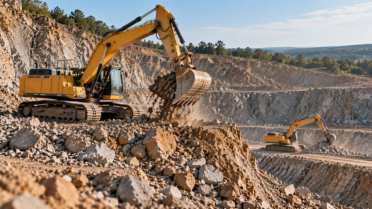
A hydraulic excavator performs a sequence of movements that appears relatively straightforward. The bucket penetrates the material, fills, rises from the excavation, swings towards a truck or stockpile, discharges its load and returns to the digging position.

Hydraulic digging force must be sufficient to penetrate the ground, while boom, stick and bucket movements need to be coordinated without unnecessary delay. Machine stability, digging depth, working radius and the position of the receiving truck all influence the time required to complete each cycle.

The engineering relationships behind these movements were examined in the preceding Machinery Spotlight feature, Why Construction Machines Look the Way They Do. Their economic consequences become apparent when the same digging cycle is repeated hundreds of times during a shift.

A truck positioned close to the excavator, at a suitable loading height, can reduce the amount of slewing required. An awkwardly positioned truck may demand a greater swing angle, extending the cycle even when material and digging conditions remain unchanged.

Consider an excavator equipped with a bucket having a nominal heaped capacity of 2.5 cubic metres. Assuming an average fill factor of 90%, each completed cycle carries approximately 2.25 loose cubic metres. This fill factor is appropriate for the assumed favourable digging conditions, rather than being representative of every material.

At a 30-second cycle time, the theoretical production rate is 120 cycles per hour, equivalent to 270 loose cubic metres. Applying a productive efficiency factor of 75% across the scheduled operating period gives an average output of 202.5 loose cubic metres per hour.

With a 36-second cycle, caused by less favourable truck positioning, increased swing distance or slower bucket filling, output falls to 168.75 loose cubic metres per hour at the same fill factor and efficiency. Over ten scheduled hours, the faster operation produces 337.5 additional loose cubic metres, representing 270 bank cubic metres of excavation at an assumed swell factor of 1.25.

The six-second increase in cycle time has reduced production by approximately 17%, while the faster arrangement delivers 20% more material than the slower one. No additional engine power, bucket capacity or machine weight is involved.

These calculations establish the basis for the opening comparison. All worked examples in this feature use stated assumptions to explain engineering and economic relationships rather than represent measured industry averages.

Real digging cycles vary with material resistance, excavation depth, hydraulic loading and operator technique. A longer cycle may also be necessary to maintain stability, avoid overloading or work safely around personnel and other equipment.

Shorter cycles do not automatically produce higher output when bucket payload changes at the same time. Research published in the peer-reviewed journal Mining in 2023, Data Analyses of Quarry Operations and Maintenance Schedules: A Production Optimization Study, examined operating data supplied by Caterpillar dealer Carter Machinery from wheel loaders working in Virginia quarries and a West Virginia coal mine.

For three of the seven quarry loaders studied, average payload increased with cycle time up to an apparent optimum of approximately 35–40 seconds. The authors suggest that operators may have spent more time filling their buckets, although this explanation was not independently measured. Results for the remaining loaders were inconclusive or anomalous, limiting how widely the finding can be applied.

The research concerns wheel loaders rather than excavators, but it illustrates a relevant production relationship: a longer digging or loading cycle may be economically worthwhile if the additional material carried more than compensates for the time required. The worked excavator comparison holds bucket fill constant to isolate the effect of cycle time. In practice, contractors need to consider both variables together, since attempting to shorten cycles by reducing bucket fill can undermine the expected production improvement.

A larger bucket can increase production where the excavator has sufficient digging capability to fill it consistently. In difficult material, an oversized bucket may achieve poor fill factors or require longer digging cycles, reducing the anticipated advantage.

Similarly, operating at excessive reach can limit effective digging force and lifting capability. A machine working from an unsuitable position may struggle to exploit its nominal performance even when it has more than enough engine power for the excavation.

Matching Haulage to Excavation

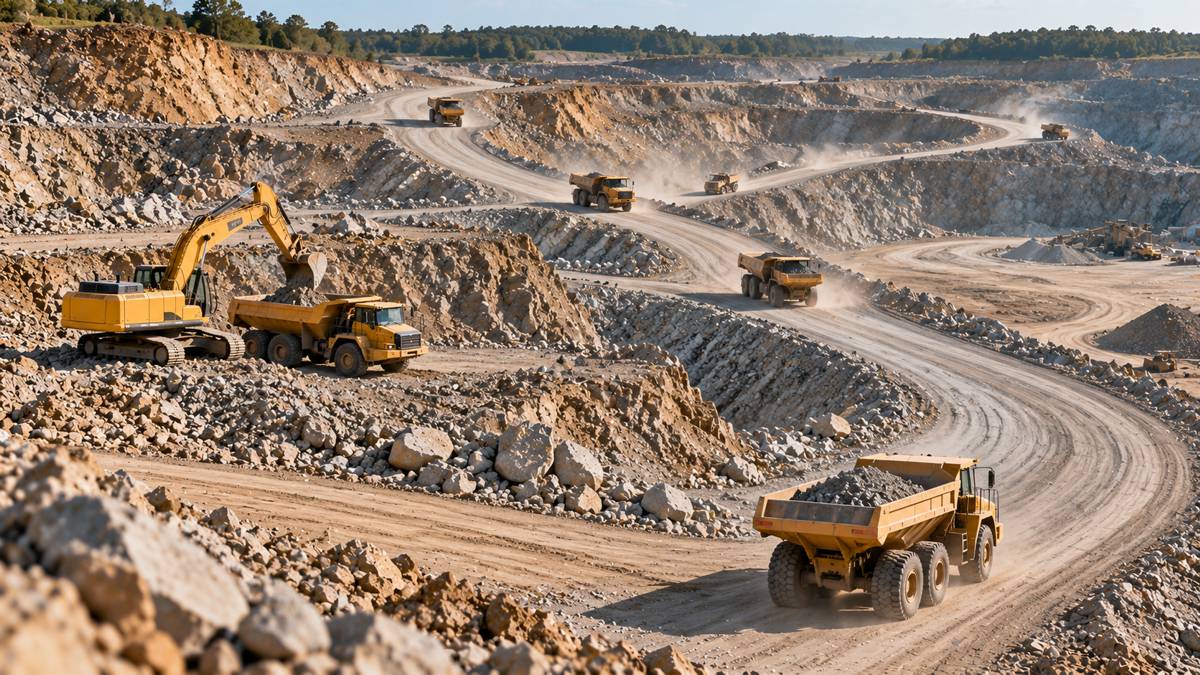
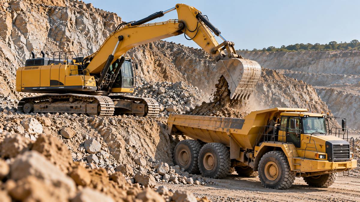
The excavator in the previous example moves approximately 2.25 loose cubic metres with each bucket. Six complete passes therefore place around 13.5 loose cubic metres into a truck, requiring three minutes of loading at a 30-second cycle time.

For a material with an assumed loose bulk density of 1.6 tonnes per cubic metre, that volume represents approximately 21.6 tonnes. The truck would need sufficient rated payload and body capacity to carry the load safely, allowing for the characteristics of the material and applicable operating limits.

If the loaded journey takes nine minutes, unloading and manoeuvring require two minutes, and the return journey takes six minutes, the complete truck cycle, including loading, is 20 minutes. Dividing the complete cycle by the three-minute loading interval produces a theoretical requirement of 6.67 trucks, making seven vehicles an initial planning estimate for maintaining continuous loading under idealised conditions.

The calculation excludes truck exchange and positioning delays at the excavator, as well as variations in travel time, loading performance and queueing. These allowances must be incorporated into a realistic fleet plan.

The relationship is commonly considered through the fleet match factor, which compares available haulage capacity with loading capacity. In a simplified single-excavator arrangement with identical trucks, the ratio of truck numbers multiplied by loading time to total truck cycle time indicates whether haulage or loading is likely to be the limiting activity.

With seven trucks operating on a 20-minute cycle, the match factor is 7 × 3 ÷ 20, or 1.05. Under the assumed conditions, the fleet has slightly more haulage capacity than the excavator requires.

A match factor below one suggests insufficient haulage capacity to keep the loading machine continuously occupied, while a value above one indicates that truck capacity exceeds the loading requirement and may create queues. Actual fleet performance is more complicated because trucks do not arrive at perfectly regular intervals, and excavators do not complete every loading cycle in precisely the same time.

Now suppose deteriorating haul-road conditions add three minutes to the loaded journey and two minutes to the return. The complete cycle increases to 25 minutes, raising the theoretical requirement to 8.33 trucks, or nine whole vehicles.

Retaining the original seven trucks reduces the match factor to 0.84. Under the simplified model, the haulage fleet can now support only approximately 84% of the excavator’s potential loading time, implying a reduction of around 16% in achievable loading output if haulage is the only constraint.

Increasing the fleet to nine trucks raises the match factor to 1.08, restoring theoretical haulage capacity at the cost of two additional vehicles. The contractor could deploy those vehicles, accept lower production or improve the haul road, with each option carrying different implications for fuel, labour, maintenance, equipment ownership and project duration.

Haul-road conditions influence the resistance that trucks encounter while travelling. Caterpillar’s rolling-resistance guidance provides indicative values for different surfaces, including approximately 1.2% for radial tyres on hard, smooth ground, 4% on rutted dirt with around 25 mm of penetration and 8% on softer ground with approximately 100 mm of penetration.

The guidance also identifies 2% as a commonly used base figure for estimating purposes. These percentages describe resistance to vehicle movement rather than direct percentage changes in fuel consumption or travel speed, with the operational effects depending on vehicle weight, available power, gradient and other conditions.

Increasing rolling resistance raises the force required to move a loaded truck. It can reduce travel speeds, increase energy demand and accelerate wear, particularly when combined with poor drainage, uneven surfaces or excessive gradients.

Caterpillar’s haul-road maintenance guidance addresses road geometry, drainage, loading areas and dumping zones, recognising that truck travel conditions affect production throughout the haulage system. A well-maintained route can shorten truck cycles and increase the frequency with which empty vehicles return to the loading face, potentially avoiding the need for additional haulage capacity.

Truck loading arrangements also influence production. A vehicle requiring an awkward final partial bucket may remain at the loading face longer than necessary, while inconsistent payloads can reduce the efficiency of the haulage fleet.

Excessive loading is not an acceptable solution. Overloading can affect tyres, braking systems, vehicle structures and haul-road safety, as well as breaching operating limits.

Fleet matching changes as projects progress, with excavation faces advancing, haul distances increasing and material destinations changing. The number of trucks required to support a loading operation at the beginning of a project may no longer be appropriate several months later.

Machine Size and Ground Conditions

Modern mining excavators, wheel loaders and high-capacity haul trucks can handle quantities of material that would once have required much larger fleets. Their advantages are most apparent in continuous bulk-production environments where equipment capacity can be used consistently.

A large excavator operating in a confined urban excavation faces different constraints. It may spend considerable time repositioning, manoeuvring around temporary supports or waiting for trucks that cannot approach the loading face efficiently. A smaller machine with better access may achieve a higher proportion of productive working time.

Ground-bearing capacity can also determine what equipment is practical. Heavy machinery operating on weak ground may require engineered working platforms or other measures to distribute loads safely, while lighter equipment may remain mobile without the same degree of preparation.

The physical characteristics of the material introduce further complications. Loose granular material may be relatively easy to excavate, although maintaining stable working faces and controlling spillage can be difficult. Cohesive soils may resist penetration, adhere to buckets and become troublesome when wet. Cemented material and rock may require ripping, hydraulic breaking or blasting before conventional excavation becomes economical.

Rock fragmentation is particularly important in bulk excavation. Well-fragmented material can allow suitable excavators and loaders to fill their buckets efficiently, while poorly fragmented material may leave voids within the bucket, require additional manipulation or produce oversize pieces that need further breaking.

Material abrasiveness affects the cost of maintaining production. Hard rock can accelerate wear on bucket teeth, cutting edges, undercarriages and other ground-engaging components. More aggressive digging techniques may improve short-term output while increasing maintenance expenditure and the likelihood of interruptions.

Moisture presents another operational variable. Some soils become easier to compact at suitable moisture contents, while excessive water can reduce bearing capacity, increase rolling resistance and make material difficult to excavate or place.

Geotechnical investigations, trial pits, boreholes and material testing help contractors anticipate these conditions. They can inform equipment selection, excavation methodology and production estimates, while identifying where dewatering, ground treatment or specialist excavation methods may be required.

Such investigations cannot eliminate geological uncertainty. Ground conditions can change between investigation locations, and unexpected obstructions or variable rock strength may still affect production. Reliable information nevertheless reduces the risk of basing equipment decisions on unrealistic assumptions.

Consider two excavators operating under broadly comparable conditions, with material quantities expressed in bank cubic metres.

	Smaller excavator	Larger excavator
Direct operating cost	£140/hour	£180/hour
Achieved production	100 bank m³/hour	180 bank m³/hour
Direct machine cost	£1.40/m³	£1.00/m³

The larger excavator costs almost 29% more per hour but achieves a direct machine cost per cubic metre approximately 29% lower. These figures exclude haulage, mobilisation, site preparation and other supporting activities, and assume the larger machine can sustain its stated production without creating congestion or exceeding the capacity of downstream operations.

A machine that appears economical when considered individually may become expensive when its requirements are imposed on the surrounding project. The appropriate choice depends on the productive capacity of the complete operation rather than machine size alone.

Equipment Reliability and Downtime

An excavator breakdown can interrupt much more than the machine itself when it occupies a critical position in a production system. If it is the only excavator loading a fleet of trucks, its failure may leave the entire haulage operation waiting. Drivers, vehicles and supporting equipment remain available, but material movement stops.

A similar effect occurs when a quarry crusher fails. Excavators and trucks may continue operating temporarily if stockpile capacity permits, although material processing eventually becomes the limiting operation.

The economic consequences extend beyond replacement components and repair labour. Idle machinery, disrupted subcontractors, delayed activities and changes to the construction programme can all increase the cost of a failure.

Maintenance planning typically combines scheduled servicing, inspections and component replacement with monitoring of actual equipment condition. Hydraulic systems are particularly important because pumps, motors, valves, cylinders, seals and hydraulic fluid are central to the performance of many construction machines.

Contamination, overheating, leakage and component wear can reduce efficiency before causing complete failure. Oil analysis, pressure monitoring, temperature measurements and diagnostic information can help maintenance teams identify developing problems, although the information is only useful when it can be interpreted correctly and the necessary maintenance performed.

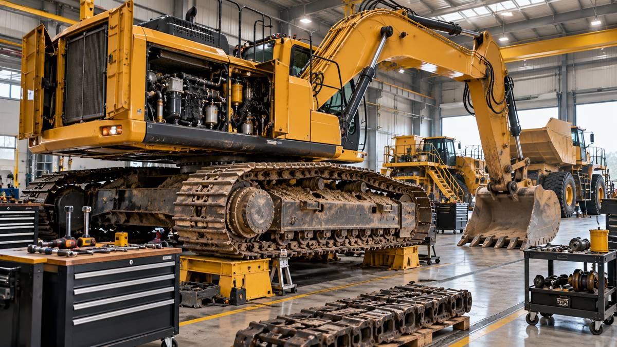
Undercarriage wear presents a different challenge. On crawler machines, tracks, rollers, idlers and sprockets operate continuously in abrasive environments. Ground conditions, travel distances, turning behaviour and maintenance practices all influence service life. Tyres play an equivalent role on wheeled equipment, where incorrect inflation, excessive loading, unsuitable road conditions and heat accumulation can affect reliability and operating costs.

A practical example of fleet maintenance planning can be found at Scotland’s Hillhouse Quarry Group. In a November 2018 Quarry Management feature published by Agg-Net, the company discussed its investment in new machinery and the rebuilding of existing prime movers following a particularly busy period that included supplying more than 800,000 tonnes of asphalt material for construction of the M8 motorway near Glasgow.

The account, which concerns a Caterpillar and Finning customer, describes a whole-life costing exercise used to guide fleet replacement and rebuilding decisions. When a machine required major work away from site, Hillhouse brought forward other repairs due within the following 12–18 months, allowing several maintenance activities to be completed during a single withdrawal from service.

This approach reduces the need for repeated machine removals, transport and subsequent interruptions, although the published account does not quantify the resulting downtime savings. Hillhouse also acquired a used dozer for approximately the cost of a few months’ hire, illustrating how equipment ownership and replacement decisions can be influenced by the expected duration of work and the cost of securing machinery when it is needed.

Equipment support arrangements are especially important in remote regions, where specialist components or technicians may take considerable time to arrive. Machinery with established local support and readily available parts can offer operational advantages that are not apparent from performance specifications.

Maintaining standby equipment can also be commercially rational despite the apparent cost of unused capacity. A reserve loader in a quarry or replacement excavator available for a critical excavation can protect production against unexpected failures.

The appropriate level of redundancy depends on the probability of breakdown, the cost of maintaining reserve capacity and the consequences of interruption. A fleet in which every machine is fully committed may appear efficient, but it can also be vulnerable to relatively minor disruption.

Operator Performance and Energy Efficiency

Construction machinery has become increasingly sophisticated, yet the operator continues to influence how effectively mechanical capability is converted into completed work. Experienced excavator operators develop an understanding of material behaviour, bucket positioning, machine balance and hydraulic response. They recognise when a bucket is cutting efficiently, when a different digging angle is required and when excessive force is unlikely to improve the result.

Smooth coordination of boom, stick, bucket and swing movements can reduce unnecessary delays and mechanical stress. On wheel loaders, efficient approaches to stockpiles, controlled bucket filling and appropriate traction management influence cycle times and tyre wear.

Bulldozer operators face similar decisions involving blade loading, cutting depth, track slip and material movement. Excessive blade loading may reduce travel speed or cause unnecessary track slip, while poorly planned material movement can create repeated handling and additional machine hours.

Operating efficiently does not mean operating as quickly as possible. Attempts to maximise cycles without regard to stability, material spillage, component loading or surrounding personnel can introduce unacceptable safety and maintenance risks.

Training and operator-assistance systems can help improve consistency. Simulators allow operators to practise equipment movements and site procedures without exposing production machinery to the same operational risks, while payload monitoring and grade-control systems provide additional information during routine work.

These technologies do not remove the need for judgement when ground conditions change or unexpected obstacles appear. Nor can they compensate for trucks being unavailable or an excavation face being poorly prepared.

A machine consuming 25 litres of diesel per hour while moving 200 cubic metres of material uses 0.125 litres per cubic metre. Another consuming 18 litres per hour while moving 100 cubic metres uses 0.18 litres per cubic metre. The first consumes more fuel each hour but approximately 31% less fuel per unit of production. Comparisons of this kind require consistent material measurements and equivalent work boundaries, particularly where machines are operating in different ground conditions or over different haul distances.

Engine idling can increase energy costs without producing useful output, particularly when equipment is waiting for trucks or other activities. Automatic engine-speed reduction and shutdown systems can reduce some of this consumption, although savings depend on duty cycle and operating practice.

Hydraulic efficiency also influences energy demand through pressure losses, throttling and heat generation. Modern control strategies attempt to improve the relationship between engine output and hydraulic demand, while selected hybrid arrangements can recover or reuse energy during suitable machine movements.

Battery-electric equipment introduces different operating considerations, particularly around charging schedules and site electrical capacity. These were examined in the first Machinery Spotlight feature, From Horsepower to Kilowatts.

The relevant economic comparison is the cost of energy per unit of useful work, together with the effects of charging or refuelling on machine availability. A lower energy price provides limited benefit if the operating arrangement creates expensive interruptions elsewhere in the production system.

Fleet Production and Material Flow

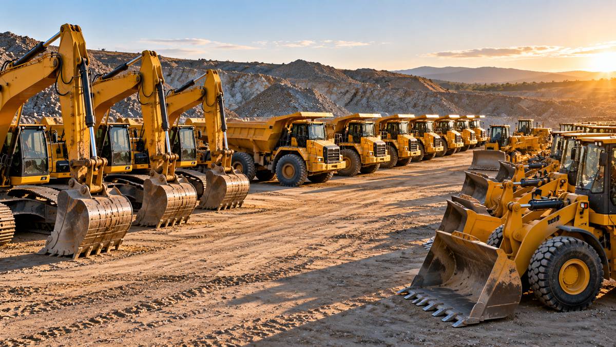
Large earthmoving operations rarely consist of excavation and haulage alone. Material may need to be ripped, excavated, transported, placed, spread, moisture-conditioned and compacted before the work is complete. Each activity has its own production capacity, and the overall operation depends on the relationship between them.

An excavator capable of producing 300 cubic metres per hour provides limited additional value if the available haulage fleet can transport only 200 cubic metres over the same period. Increasing excavation capacity without addressing the haulage constraint creates additional waiting time.

The same relationship applies further along the process. Trucks may deliver material faster than dozers can spread it or compactors can achieve the specified density, causing material to accumulate and disrupting the intended construction sequence.

Stockpiles can provide a useful buffer between operations, allowing excavation or processing to continue temporarily when downstream activities are interrupted. However, stockpiling introduces additional handling costs, space requirements and material-management considerations.

Compaction demonstrates why measuring material movement alone can be insufficient. A contractor constructing an embankment must deliver material placed to the required geometry, moisture condition and density. Transporting additional tonnes to the embankment creates little value if placement and compaction cannot accommodate them.

Excessively thick lifts, unsuitable moisture content or inadequate compaction may result in reworking and testing delays, consuming further machine hours. The relevant production measure is therefore the quantity of acceptable completed work, rather than the amount of material handled at an individual stage.

The same principle applies to grading. A dozer may move large quantities of material rapidly, but repeated correction of levels consumes time and fuel. Accurate survey information and suitable machine-control systems can reduce unnecessary reworking where the underlying design data are reliable.

Versatile equipment can help contractors balance changing workloads, although the commercial trade-offs between multipurpose machinery and dedicated equipment were examined in Why Construction Machines Look the Way They Do, including its discussion of the backhoe loader. An excavator using several attachments may reduce mobilisation requirements on a varied project, while a dedicated machine may be more productive where one activity dominates the workload.

The economic comparison depends on how effectively each option contributes to the complete production sequence. Contractors must also consider equipment utilisation across several projects, since a machine achieving modest utilisation on one site may deliver excellent annual utilisation when transferred efficiently between contracts.

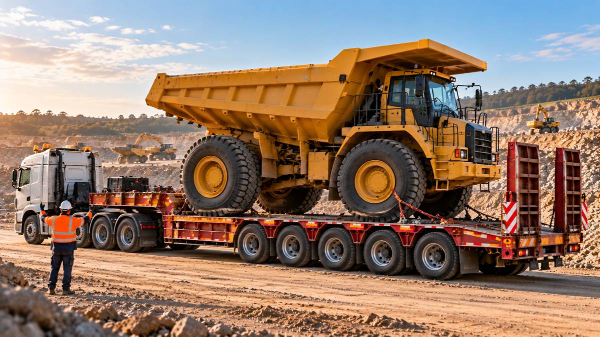
Transport costs, mobilisation time and maintenance commitments can reduce the benefit of frequent redeployment. Fleet planning consequently operates across different time horizons, from hourly production and weekly construction targets to annual equipment utilisation and the availability of machinery for future work.

Digital Production Measurement

Historically, contractors relied on operator reports, engine-hour meters, fuel records, survey measurements and manual production logs to understand equipment performance. Connected machinery can now provide more detailed operating information, including location, fuel consumption, idle time, fault codes, payload measurements and selected performance parameters.

An excavator showing high engine utilisation may appear productive until cycle analysis reveals long waiting periods or excessive time spent repositioning. A haulage fleet may accumulate substantial operating hours while delivering relatively few tonnes because of congestion or poorly coordinated dispatching.

Payload systems can help contractors assess whether trucks are consistently loaded within permitted limits. GNSS positioning and digital terrain models can support measurement of excavation progress, while machine-control systems can reduce reliance on repeated manual setting-out.

Survey data can establish the amount of material removed from an excavation or placed within an embankment. Machine records can then help explain the equipment time and energy required to achieve that result.

However, machine manufacturers may use different definitions of utilisation, idling and productive time. Sensor measurements can be affected by calibration, operating conditions and technological limitations, while proprietary platforms can complicate the integration of information from mixed fleets.

An excavator may be stationary because its operator is waiting unnecessarily, but it may also be waiting for a survey check, safety clearance or another essential activity. An increase in average cycle time may indicate inefficient working geometry, harder material, deeper excavation or a deliberate change in operating technique.

A machine-control system may record excavation progress without establishing whether the completed work meets every specification. Survey verification, material testing and quality assurance remain necessary where required by the project.

Better data can nevertheless help contractors identify opportunities to improve production using existing machinery. More consistent loading, reduced unnecessary idling, improved haul-road maintenance and better coordination between machines can all affect the cost of completed work.

Coordinated Fleet Operations

Autonomous haulage provides an established commercial example of machinery being coordinated through centralised control systems, particularly in large mining operations with defined routes and managed traffic conditions. In April 2026, Komatsu reported that its FrontRunner autonomous haulage system had reached 1,000 commissioned ultra-class autonomous trucks.

The milestone was examined in the first Machinery Spotlight feature. Komatsu is extending automation beyond haulage to activities including road maintenance, with autonomous water trucks forming part of its wider development programme.

Water trucks perform an essential supporting function on many haul roads, particularly where dust suppression is required to maintain visibility and suitable operating conditions. Their deployment must be coordinated with haulage movements, road maintenance and site requirements.

Caterpillar’s haul-road guidance recognises that watering must be carefully managed. Insufficient watering can allow dust to affect visibility and vehicle operating conditions, while excessive water can soften the road surface, increase rolling resistance and reduce travel speeds.

Coordinating water-truck movements therefore involves balancing dust suppression against the effects of additional moisture on haulage performance. Autonomous watering may eventually support more consistent management of this relationship, although its economic benefits depend on the operating environment and the effectiveness of the complete system.

Komatsu is also pursuing a software-defined vehicle strategy intended to support greater integration between machinery, autonomy systems and fleet management. The company describes this as part of its next generation of autonomous mining equipment, although the commercial maturity of individual capabilities varies.

Connected fleet systems could adjust truck dispatching as haul distances change, identify when road maintenance would provide a better return than additional haulage capacity or schedule maintenance around planned production interruptions. Digital simulations may also allow contractors to evaluate alternative fleet arrangements before moving equipment, assessing changes to haul routes, excavation sequences or machine positions against expected production, operating costs and site constraints.

Such approaches depend on accurate data, realistic models and appropriate operational safeguards. Construction sites are less predictable than many established autonomous mining environments, with frequently changing work areas, temporary obstacles and interactions between machinery, personnel and subcontractors.

Better-informed coordination of equipment and production activities is already relevant to contractors operating conventional fleets. Autonomy can extend those capabilities where operating conditions and safety arrangements permit, but the underlying requirements for reliable production information and coordinated material movement remain unchanged.

Production Economics and Fleet Investment

The two excavators at the beginning of this article possess identical mechanical capabilities. Their different economic outcomes arise from the conditions in which they operate and the effectiveness of the production systems supporting them.

One benefits from efficient loading geometry, reliable truck availability and prepared working conditions. The other loses time through interruptions, unnecessary movements and inconsistent material flow.

Improving the second operation may require relatively little investment in machinery. Repositioning trucks, maintaining the haul road, adjusting the excavation sequence or improving dispatching could deliver greater production without changing the excavator itself.

Across larger fleets, these decisions influence the amount of capital required, the energy consumed and the time needed to complete a project. Equipment manufacturers will continue developing more powerful, efficient and intelligent machinery, while connected systems offer increasingly detailed information about how that equipment is used.

Before committing capital to additional equipment, contractors need to establish whether existing machinery has reached the limits of its productive capability or whether the surrounding operation is preventing it from achieving those limits. An additional excavator may increase production where excavation capacity is genuinely the constraint. Where trucks are already queuing, haul roads are deteriorating or placement operations cannot accommodate more material, the same investment may simply add another machine to an inefficient system.

The most economical improvement may be a larger machine, a better-matched fleet or a change in working method. Establishing which one is required begins with measuring the work actually completed and identifying where production is being lost.

Key Industry Questions

1. How is excavator productivity calculated? A basic estimate multiplies digging cycles per hour by average bucket payload and an appropriate productive-efficiency factor. The resulting production should use a consistent material-volume basis.
2. What is the difference between bank and loose cubic metres? Bank volume measures material in its undisturbed condition, while loose volume measures it after excavation. Excavation generally increases volume through swelling, requiring a conversion factor when comparing quantities.
3. How many haul trucks are needed for one excavator? A preliminary estimate divides the complete truck cycle time by the loading interval. Actual fleet requirements must also account for queueing, payload, traffic, delays and operating variability.
4. What is the fleet match factor? It expresses the relationship between haulage capacity and loading capacity. In a simplified fleet, it helps indicate whether trucks are likely to queue or the loading machine is likely to wait.
5. Does a larger excavator always have a lower cost per cubic metre? No. Larger equipment may achieve lower unit costs when effectively utilised, but constrained access, inadequate haulage capacity and additional support requirements can reduce its economic advantage.
6. Why does haul-road maintenance affect productivity? Poor road conditions increase rolling resistance, reduce travel speeds and can accelerate tyre and component wear. Longer truck cycles may reduce excavation throughput or require additional haulage equipment.
7. What is the difference between machine availability and utilisation? Availability describes the proportion of relevant time a machine is fit to work, while utilisation measures how much of that time it is used. Neither alone establishes useful production.
8. Can electric construction machinery reduce earthmoving costs? Potentially, depending on energy prices, duty cycles, equipment performance and charging arrangements. Comparisons should consider total production costs rather than energy consumption alone.
9. How can telematics improve construction equipment productivity? Telematics can reveal idle time, operating patterns, fuel consumption and equipment-health information. Improvements depend on interpreting those records alongside actual work completed.
10. Will autonomous equipment eliminate the need for fleet planning? No. Automated machines still require coordinated loading, transport, material handling, maintenance and safe operating arrangements. Automation may improve fleet coordination but does not remove physical production constraints.

Strategic Takeaways

1. Production should be measured in completed work. Engine hours and nominal machine capacities provide limited insight without reliable output measurements.
2. Fleet balance determines achievable throughput. Additional excavation capacity has little value when haulage, placement or compaction is already the limiting operation.
3. Working conditions are economic variables. Material characteristics, haul-road quality, machine positioning and site preparation directly influence production costs.
4. Reliability protects the entire operation. Critical equipment failures can create financial consequences far beyond the cost of repairing the affected machine.
5. Fleet investment should follow operational diagnosis. Improving haulage coordination, maintenance or site organisation may provide a better return than purchasing additional machinery.